本文最后更新于:July 15, 2022 am
21年全国大学生计算机应用能力与信息素养大赛 注:此代码实现过程仅是本人初学后所敲,很多地方不足,仅供大家参考。 因为大赛结束后就没有赛题及相关介绍,这里提供给大家
代码如下: 1 2 3 4 5 6 7 import numpy as npimport pandas as pdimport matplotlib.pyplot as pltimport seaborn as sns'C:/Users/86155/Desktop/大数据竞赛数据集_本科组.csv' )
X0
X1
X2
X3
X4
X5
X6
X7
X8
X9
X10
X11
X12
X13
X14
0
1/1/2015
Quarter1
sweing
Thursday
8
0.80
26.16
1108.0
7080
98
0.0
0
0
59.0
0.940725
1
1/1/2015
Quarter1
finishing
Thursday
1
0.75
3.94
NaN
960
0
0.0
0
0
8.0
0.886500
2
1/1/2015
Quarter1
sweing
Thursday
11
0.80
11.41
968.0
3660
50
0.0
0
0
30.5
0.800570
3
1/1/2015
Quarter1
sweing
Thursday
12
0.80
11.41
968.0
3660
50
0.0
0
0
30.5
0.800570
4
1/1/2015
Quarter1
sweing
Thursday
6
0.80
25.90
1170.0
1920
50
0.0
0
0
56.0
0.800382
1 2 3 4 5 6 7 8 import pandas as pd'C:/Users/86155/Desktop/xinguan.xlsx' )
城市
累计确诊
现有疑似
累计死亡
经度
纬度
0
北京
1651
0
9
116.46
39.92
1
天津
1372
0
3
117.20
39.12
2
河北
1671
0
7
114.52
38.05
3
山西
295
0
0
112.55
37.87
4
内蒙古
1666
0
1
111.73
40.83
<class 'pandas.core.frame.DataFrame'>
RangeIndex: 1197 entries, 0 to 1196
Data columns (total 15 columns):
# Column Non-Null Count Dtype
--- ------ -------------- -----
0 X0 1197 non-null datetime64[ns]
1 X1 1197 non-null object
2 X2 1197 non-null object
3 X3 1197 non-null object
4 X4 1197 non-null int64
5 X5 1197 non-null float64
6 X6 1197 non-null float64
7 X7 691 non-null float64
8 X8 1197 non-null int64
9 X9 1197 non-null int64
10 X10 1197 non-null float64
11 X11 1197 non-null int64
12 X12 1197 non-null int64
13 X13 1197 non-null float64
14 X14 1197 non-null float64
dtypes: datetime64[ns](1), float64(6), int64(5), object(3)
memory usage: 140.4+ KB
X0
X1
X2
X3
X4
X5
X6
X7
X8
X9
X10
X11
X12
X13
X14
0
False
False
False
False
False
False
False
False
False
False
False
False
False
False
False
1
False
False
False
False
False
False
False
False
False
False
False
False
False
False
False
2
False
False
False
False
False
False
False
False
False
False
False
False
False
False
False
3
False
False
False
False
False
False
False
False
False
False
False
False
False
False
False
4
False
False
False
False
False
False
False
False
False
False
False
False
False
False
False
...
...
...
...
...
...
...
...
...
...
...
...
...
...
...
...
1192
False
False
False
False
False
False
False
False
False
False
False
False
False
False
False
1193
False
False
False
False
False
False
False
False
False
False
False
False
False
False
False
1194
False
False
False
False
False
False
False
False
False
False
False
False
False
False
False
1195
False
False
False
False
False
False
False
False
False
False
False
False
False
False
False
1196
False
False
False
False
False
False
False
False
False
False
False
False
False
False
False
1197 rows × 15 columns
X0 datetime64[ns]
X1 object
X2 object
X3 object
X4 int64
X5 float64
X6 float64
X7 float64
X8 int64
X9 int64
X10 float64
X11 int64
X12 int64
X13 float64
X14 float64
dtype: object
1 2 'X7' ]=data['X7' ].fillna(data['X7' ].median())
X4
X5
X6
X7
X8
X9
X10
X11
X12
X13
X14
count
1197.000000
1197.000000
1197.000000
1197.000000
1197.000000
1197.000000
1197.000000
1197.000000
1197.000000
1197.000000
1197.000000
mean
6.426901
0.729632
15.062172
1126.437761
4567.460317
38.210526
0.730159
0.369256
0.150376
34.609858
0.735091
std
3.463963
0.097891
10.943219
1397.653191
3348.823563
160.182643
12.709757
3.268987
0.427848
22.197687
0.174488
min
1.000000
0.070000
2.900000
7.000000
0.000000
0.000000
0.000000
0.000000
0.000000
2.000000
0.233705
25%
3.000000
0.700000
3.940000
970.000000
1440.000000
0.000000
0.000000
0.000000
0.000000
9.000000
0.650307
50%
6.000000
0.750000
15.260000
1039.000000
3960.000000
0.000000
0.000000
0.000000
0.000000
34.000000
0.773333
75%
9.000000
0.800000
24.260000
1083.000000
6960.000000
50.000000
0.000000
0.000000
0.000000
57.000000
0.850253
max
12.000000
0.800000
54.560000
23122.000000
25920.000000
3600.000000
300.000000
45.000000
2.000000
89.000000
1.120437
1 2 3 4 5
0 False
1 False
2 False
3 False
4 False
...
1192 False
1193 False
1194 False
1195 False
1196 False
Length: 1197, dtype: bool
X0
X1
X2
X3
X4
X5
X6
X7
X8
X9
X10
X11
X12
X13
X14
0
1/1/2015
Quarter1
sweing
Thursday
8
0.80
26.16
1108.0
7080
98
0.0
0
0
59.0
0.940725
1
1/1/2015
Quarter1
finishing
Thursday
1
0.75
3.94
1039.0
960
0
0.0
0
0
8.0
0.886500
2
1/1/2015
Quarter1
sweing
Thursday
11
0.80
11.41
968.0
3660
50
0.0
0
0
30.5
0.800570
3
1/1/2015
Quarter1
sweing
Thursday
12
0.80
11.41
968.0
3660
50
0.0
0
0
30.5
0.800570
4
1/1/2015
Quarter1
sweing
Thursday
6
0.80
25.90
1170.0
1920
50
0.0
0
0
56.0
0.800382
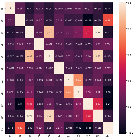
1 2 3 4 5 6 7 import seaborn as sns'font.sans-serif' ]='SimHei' 'X0' ,'X1' ,'X2' ,'X3' ,'X4' ,'X5' ,'X6' ,'X7' ,'X8' ,'X9' ,'X10' ,'X11' ,'X12' ,'X13' ,'X14' ]].corr()10 ,10 )) 0.8 ,annot=True )
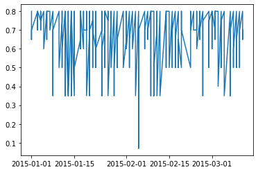
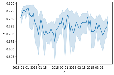
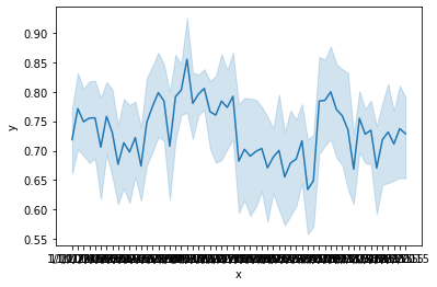
1 2 x = data['X0' ]'X5' ]
1 2 3 4 5 6 7 8 9 10 plt.plot(x,y)'x' :x,'y' :y'x' ,y='y' ,data=df)
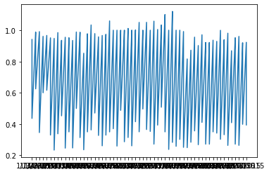
1 2 x = data['X0' ]'X14' ]
1 2 3 4 5 6 7 8 9 10 plt.plot(x,y)'x' :x,'y' :y'x' ,y='y' ,data=df)
X0
X1
X2
X3
X4
X5
X6
X7
X8
X9
X10
X11
X12
X13
X14
0
1/1/2015
Quarter1
sweing
Thursday
8
0.80
26.16
1108.0
7080
98
0.0
0
0
59.0
0.940725
1
1/1/2015
Quarter1
finishing
Thursday
1
0.75
3.94
NaN
960
0
0.0
0
0
8.0
0.886500
2
1/1/2015
Quarter1
sweing
Thursday
11
0.80
11.41
968.0
3660
50
0.0
0
0
30.5
0.800570
3
1/1/2015
Quarter1
sweing
Thursday
12
0.80
11.41
968.0
3660
50
0.0
0
0
30.5
0.800570
4
1/1/2015
Quarter1
sweing
Thursday
6
0.80
25.90
1170.0
1920
50
0.0
0
0
56.0
0.800382
array([ 8, 1, 11, 12, 6, 7, 2, 3, 9, 10, 5, 4], dtype=int64)
1 2 'X0' ,'X1' ,'X2' ,'X3' ],axis=1 )
X4
X5
X6
X7
X8
X9
X10
X11
X12
X13
X14
0
8
0.80
26.16
1108.0
7080
98
0.0
0
0
59.0
0.940725
1
1
0.75
3.94
1039.0
960
0
0.0
0
0
8.0
0.886500
2
11
0.80
11.41
968.0
3660
50
0.0
0
0
30.5
0.800570
3
12
0.80
11.41
968.0
3660
50
0.0
0
0
30.5
0.800570
4
6
0.80
25.90
1170.0
1920
50
0.0
0
0
56.0
0.800382
1 2 3 4 5 6 7 8 9 10 11 from sklearn.cluster import KMeansfrom sklearn.preprocessing import scalerange (1 ,20 )for k in k_range:
[13167.000000000002,
10368.001747788787,
8985.612362104612,
7956.326143721504,
6934.1999209667265,
6364.89500698171,
5600.08786819714,
4740.428352871961,
4360.332443867376,
3918.830271323268,
3613.3367590027497,
3302.354785621584,
3095.576217636003,
2963.791234943202,
2686.863451514291,
2584.874003399748,
2427.534059702044,
2337.8239778345887,
2250.377455323783]
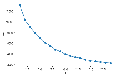
1 2 3 4 5 6 7 8 9 10 11 12 13 14 15 16 from sklearn.cluster import KMeansimport matplotlib.pyplot as pltfor k in range (1 ,20 ):'X4' , 'X14' ]])range (1 ,20 )'k' )'sse' )'o-' )
1 data2 = data1[['X4' ,'X14' ]]
1 2 3 4 5 5 )
array([4, 0, 3, ..., 4, 1, 4])
1 2 3
array([[ 1.50934579, 0.7954856 ],
[ 9.49019608, 0.72724343],
[ 3.99317406, 0.75813807],
[11.52941176, 0.73337501],
[ 7.05016722, 0.67570864]])
1 2 3 4 5 6 'X4' , 'X14' ]
X4
X14
0
1.509346
0.795486
1
9.490196
0.727243
2
3.993174
0.758138
3
11.529412
0.733375
4
7.050167
0.675709
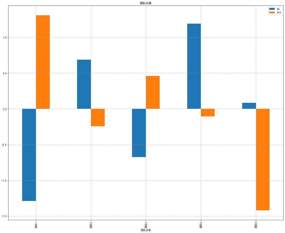
1 2 3 0 ))/(result.std(axis=0 ))
X4
X14
0
-1.286294
1.308114
1
0.685944
-0.244505
2
-0.672487
0.458397
3
1.189877
-0.105002
4
0.082961
-1.417004
1 2 3 4 5 6 7 plt.rcParams['font.sans-serif' ] = ['SimHei' ]'axes.unicode_minus' ] = False '团队分类' ]=list (['团队1' ,'团队2' ,'团队3' ,'团队4' ,'团队5' ]) 20 ,16 ),x='团队分类' ,title='团队分类' ,legend='beast' )'--' )11 )
<matplotlib.legend.Legend at 0x290ef9f0940>
1 2 3 4 5 6 7 8 9 10 from sklearn.preprocessing import scalerange (1 ,20 )for k in k_range:
[13167.000000000002,
10368.001747788787,
9059.320705761347,
7910.63025239119,
6956.651138200236,
6077.878903205976,
5511.898303743294,
4795.324291351495,
4429.152799214559,
3906.8041968464554,
3603.2482162246365,
3316.165899966484,
3147.436870420017,
2878.2859554852253,
2684.5121690958435,
2563.069034412572,
2421.7083978310657,
2315.6588424369897,
2228.865852777383]
1 2 3 4 5 6 7 8 9 10 11 12 13 14 15 import pandas as pdfrom sklearn.cluster import KMeansimport matplotlib.pyplot as pltfor k in range (1 ,20 ):'X4' ,'X5' ,'X6' ,'X7' ,'X8' ,'X9' ,'X10' ,'X11' ,'X12' ,'X13' ,'X14' ]])range (1 ,20 )'k' )'sse' )'o-' )
1 2 3 4 5 5 )
array([1, 4, 0, ..., 4, 4, 4])
1 2 3
array([[ 7.64179104e+00, 7.33582090e-01, 1.41852239e+01,
9.67542289e+02, 3.75223881e+03, 2.67114428e+01,
2.23880597e-02, 1.49253731e-01, 2.43781095e-01,
3.34527363e+01, 7.22864179e-01],
[ 5.97450425e+00, 7.15212465e-01, 2.35174788e+01,
1.06944476e+03, 6.65855524e+03, 4.08356941e+01,
2.37960340e+00, 7.13881020e-01, 3.03116147e-01,
5.24617564e+01, 7.15187532e-01],
[ 5.93333333e+00, 7.23939394e-01, 2.39216364e+01,
1.08087273e+03, 1.05087273e+04, 4.88242424e+01,
7.77156117e-16, 7.21644966e-16, -1.66533454e-16,
5.49757576e+01, 7.34676496e-01],
[ 5.33333333e+00, 8.00000000e-01, 2.13800000e+01,
1.94093333e+04, 6.19000000e+03, 7.86666667e+01,
1.11022302e-16, 0.00000000e+00, 0.00000000e+00,
5.35833333e+01, 8.83637858e-01],
[ 6.43432203e+00, 7.39830508e-01, 5.93468220e+00,
1.02024576e+03, 1.25317797e+03, 3.69194915e+01,
6.25000000e-02, 3.38983051e-01, 5.08474576e-02,
1.43908898e+01, 7.53440033e-01]])
1 2 3 4 5 6 'X4' ,'X5' ,'X6' ,'X7' ,'X8' ,'X9' ,'X10' ,'X11' ,'X12' ,'X13' ,'X14' ]
X4
X5
X6
X7
X8
X9
X10
X11
X12
X13
X14
0
7.641791
0.733582
14.185224
967.542289
3752.238806
26.711443
2.238806e-02
1.492537e-01
2.437811e-01
33.452736
0.722864
1
5.974504
0.715212
23.517479
1069.444759
6658.555241
40.835694
2.379603e+00
7.138810e-01
3.031161e-01
52.461756
0.715188
2
5.933333
0.723939
23.921636
1080.872727
10508.727273
48.824242
7.771561e-16
7.216450e-16
-1.665335e-16
54.975758
0.734676
3
5.333333
0.800000
21.380000
19409.333333
6190.000000
78.666667
1.110223e-16
0.000000e+00
0.000000e+00
53.583333
0.883638
4
6.434322
0.739831
5.934682
1020.245763
1253.177966
36.919492
6.250000e-02
3.389831e-01
5.084746e-02
14.390890
0.753440
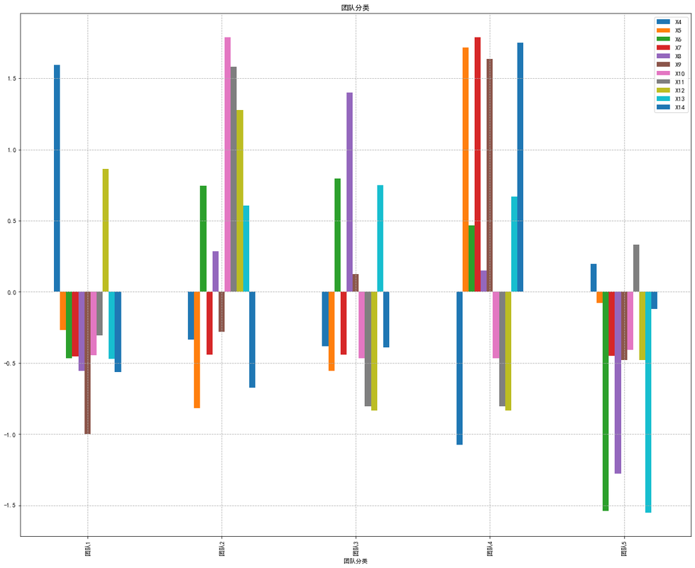
1 2 3 0 ))/(result.std(axis=0 ))
X4
X5
X6
X7
X8
X9
X10
X11
X12
X13
X14
0
1.595128
-0.266799
-0.468191
-0.455358
-0.555229
-0.997981
-0.445977
-0.304834
0.865386
-0.471215
-0.562291
1
-0.334401
-0.815573
0.744629
-0.442958
0.285093
-0.281737
1.788331
1.583047
1.278707
0.605367
-0.672696
2
-0.382048
-0.554865
0.797153
-0.441567
1.398317
0.123365
-0.467198
-0.803878
-0.832763
0.747749
-0.392407
3
-1.076420
1.717371
0.466842
1.788828
0.149616
1.636681
-0.467198
-0.803878
-0.832763
0.668888
1.749945
4
0.197740
-0.080134
-1.540432
-0.448945
-1.277798
-0.480328
-0.407957
0.329542
-0.478566
-1.550789
-0.122551
1 2 3 4 5 6 7 plt.rcParams['font.sans-serif' ] = ['SimHei' ]'axes.unicode_minus' ] = False '团队分类' ]=list (['团队1' ,'团队2' ,'团队3' ,'团队4' ,'团队5' ]) 20 ,16 ),x='团队分类' ,title='团队分类' ,legend='beast' )'--' )11 )
<matplotlib.legend.Legend at 0x290efa33780>
1 2 3 'X0' ] = pd.to_datetime(data['X0' ], format ='%m/%d/%Y' )
1 2 3 4 import datetime2015 ,1 ,1 )2015 ,3 ,1 )
1 2 3 subset = data[data['X0' ]>=start]'X0' ]<=end]
(1005, 15)
X0
X1
X2
X3
X4
X5
X6
X7
X8
X9
X10
X11
X12
X13
X14
0
2015-01-01
Quarter1
sweing
Thursday
8
0.80
26.16
1108.0
7080
98
0.0
0
0
59.0
0.940725
1
2015-01-01
Quarter1
finishing
Thursday
1
0.75
3.94
1039.0
960
0
0.0
0
0
8.0
0.886500
2
2015-01-01
Quarter1
sweing
Thursday
11
0.80
11.41
968.0
3660
50
0.0
0
0
30.5
0.800570
3
2015-01-01
Quarter1
sweing
Thursday
12
0.80
11.41
968.0
3660
50
0.0
0
0
30.5
0.800570
4
2015-01-01
Quarter1
sweing
Thursday
6
0.80
25.90
1170.0
1920
50
0.0
0
0
56.0
0.800382
...
...
...
...
...
...
...
...
...
...
...
...
...
...
...
...
1000
2015-03-01
Quarter1
finishing
Sunday
2
0.70
3.90
1039.0
960
0
0.0
0
0
8.0
0.585000
1001
2015-03-01
Quarter1
sweing
Sunday
7
0.80
30.10
934.0
6960
0
3.5
15
0
58.0
0.579511
1002
2015-03-01
Quarter1
finishing
Sunday
1
0.60
3.94
1039.0
3360
0
0.0
0
0
8.0
0.448722
1003
2015-03-01
Quarter1
finishing
Sunday
9
0.75
2.90
1039.0
960
0
0.0
0
0
8.0
0.447083
1004
2015-03-01
Quarter1
finishing
Sunday
7
0.80
4.60
1039.0
3360
0
0.0
0
0
8.0
0.350417
1005 rows × 15 columns
array(['sweing', 'finishing ', 'finishing'], dtype=object)
1 2 data4=data3.drop(['X0' ,'X1' ,'X2' ,'X3' ],axis=1 )
X4
X5
X6
X7
X8
X9
X10
X11
X12
X13
X14
0
8
0.80
26.16
1108.0
7080
98
0.0
0
0
59.0
0.940725
1
1
0.75
3.94
1039.0
960
0
0.0
0
0
8.0
0.886500
2
11
0.80
11.41
968.0
3660
50
0.0
0
0
30.5
0.800570
3
12
0.80
11.41
968.0
3660
50
0.0
0
0
30.5
0.800570
4
6
0.80
25.90
1170.0
1920
50
0.0
0
0
56.0
0.800382
1 2 3 4 5 'X14' ], axis = 1 )
(1005, 10)
1 2 3 4 from sklearn.model_selection import train_test_split6 )
1 2 3 4 5 6 from sklearn.preprocessing import StandardScaler
1 2 3 4 5 6 from sklearn.linear_model import LogisticRegression 'int' ))
LogisticRegression()
1 2 3 4 5 6 1.0 , class_weight=None , dual=False , fit_intercept=True ,1 , max_iter=100 , multi_class='ovr' , n_jobs=1 ,'l2' , random_state=None , solver='liblinear' , tol=0.0001 ,0 , warm_start=False )
LogisticRegression(multi_class='ovr', n_jobs=1, solver='liblinear')
1 log_reg.score(X_train,y_train.astype('int' ))
0.9867197875166003
1 log_reg.score(X_test,y_test.astype('int' ))
0.9761904761904762
1 2 3 4 5 6 7 8 from sklearn.metrics import accuracy_score'int' ),y_predict_log)
0.9761904761904762
1 2 3 4 5 6 7 8 9 10 'C' :[0.01 ,0.1 ,1 ,10 ,100 ],'penalty' :['l2' ,'l1' ],'class_weight' :['balanced' ,None ]
1 2 3 4 from sklearn.model_selection import GridSearchCV10 ,n_jobs=-1 )
1 2 %%time'int' ))
Wall time: 1.69 s
GridSearchCV(cv=10, estimator=LogisticRegression(), n_jobs=-1,
param_grid=[{'C': [0.01, 0.1, 1, 10, 100],
'class_weight': ['balanced', None],
'penalty': ['l2', 'l1']}])
1 2 3
LogisticRegression(C=1)
1 2 3 4 LogisticRegression(C=0.01 , class_weight=None , dual=False , fit_intercept=True ,1 , max_iter=100 , multi_class='ovr' , n_jobs=1 ,'l2' , random_state=None , solver='liblinear' , tol=0.0001 ,0 , warm_start=False )
LogisticRegression(C=0.01, multi_class='ovr', n_jobs=1, solver='liblinear')
1 2 3
0.9853859649122807
1 2 3
{'C': 1, 'class_weight': None, 'penalty': 'l2'}
1 2 log_reg = grid_search.best_estimator_'int' ))
0.9867197875166003
1 log_reg.score(X_test,y_test.astype('int' ))
0.9761904761904762
1 2 3 4 5 6 7 from sklearn.metrics import f1_score'int' ),y_predict_log)
0.5
1 2 3 4 5 from sklearn.metrics import classification_reportprint (classification_report(y_test.astype('int' ),y_predict_log))
precision recall f1-score support
0 0.98 1.00 0.99 244
1 0.75 0.38 0.50 8
accuracy 0.98 252
macro avg 0.86 0.69 0.74 252
weighted avg 0.97 0.98 0.97 252
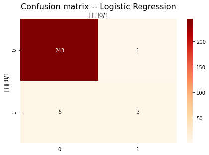
1 2 3 4 5 from sklearn.metrics import confusion_matrix'int' ),y_predict_log)
array([[243, 1],
[ 5, 3]], dtype=int64)
1 2 3 4 5 6 7 8 9 10 11 12 13 14 15 16 17 18 def plot_cnf_matirx (cnf_matrix,description ):0 ,1 ]len (class_names))True , cmap = 'OrRd' ,'g' )'top' )1.1 ,fontsize=16 )'实际值0/1' ,fontsize=12 )'预测值0/1' ,fontsize=12 )'Confusion matrix -- Logistic Regression' )
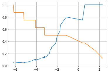
1 2 3 4 5 6 decision_scores = log_reg.decision_function(X_test)from sklearn.metrics import precision_recall_curve'int' ),decision_scores)
1 2 3 4 5 6 1 ])1 ])
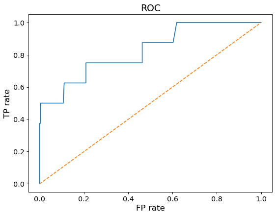
1 2 3 4 5 from sklearn.metrics import roc_curve'int' ),decision_scores)
1 2 3 4 5 6 7 8 9 10 11 12 def plot_roc_curve (fprs,tprs ):8 ,6 ),dpi=80 )0 ,1 ],linestyle='--' )13 )13 )'TP rate' ,fontsize=15 )'FP rate' ,fontsize=15 )'ROC' ,fontsize=17 )
1 2 3 4 from sklearn.metrics import roc_auc_score 'int' ),decision_scores)
0.825563524590164
逻辑回归模型得分0.82556 1 2 3 4 5 6 7 8 9 10 11 12 13 'weights' :['uniform' ],'n_neighbors' :[i for i in range (1 ,31 )]'weights' :['distance' ],'n_neighbors' :[i for i in range (1 ,31 )],'p' :[i for i in range (1 ,6 )]
1 2 3 4 5 6 7 %%timefrom sklearn.neighbors import KNeighborsClassifier'int' ))
Wall time: 14.3 s
GridSearchCV(estimator=KNeighborsClassifier(),
param_grid=[{'n_neighbors': [1, 2, 3, 4, 5, 6, 7, 8, 9, 10, 11, 12,
13, 14, 15, 16, 17, 18, 19, 20, 21,
22, 23, 24, 25, 26, 27, 28, 29, 30],
'weights': ['uniform']},
{'n_neighbors': [1, 2, 3, 4, 5, 6, 7, 8, 9, 10, 11, 12,
13, 14, 15, 16, 17, 18, 19, 20, 21,
22, 23, 24, 25, 26, 27, 28, 29, 30],
'p': [1, 2, 3, 4, 5], 'weights': ['distance']}])
1 grid_search.best_estimator_
KNeighborsClassifier(n_neighbors=3)
1 2 3 KNeighborsClassifier(algorithm='auto' , leaf_size=30 , metric='minkowski' ,None , n_jobs=1 , n_neighbors=24 , p=3 ,'distance' )
KNeighborsClassifier(n_jobs=1, n_neighbors=24, p=3, weights='distance')
0.9840618101545253
1 grid_search.best_params_
{'n_neighbors': 3, 'weights': 'uniform'}
1 2 knn_clf = grid_search.best_estimator_'int' ))
0.9853917662682603
1 knn_clf.score(X_test,y_test.astype('int' ))
0.9801587301587301
1 y_predict_knn = knn_clf.predict(X_test)
1 2 3 'int' ),y_predict_knn)
0.5454545454545454
1 print (classification_report(y_test.astype('int' ),y_predict_knn))
precision recall f1-score support
0 0.98 1.00 0.99 244
1 1.00 0.38 0.55 8
accuracy 0.98 252
macro avg 0.99 0.69 0.77 252
weighted avg 0.98 0.98 0.98 252
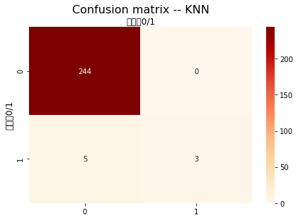
1 2 3 4 'int' ),y_predict_knn)
array([[244, 0],
[ 5, 3]], dtype=int64)
1 2 'Confusion matrix -- KNN' )
1 2 3 4 5 6 7 8 9 10 11 12 1 ]from sklearn.metrics import precision_recall_curve'int' ),y_probabilities)1 ])1 ])
1 2 3 4 5 6 from sklearn.metrics import roc_curve'int' ),decision_scores)
1 2 3 4 from sklearn.metrics import roc_auc_score 'int' ),y_probabilities)
0.7984118852459017
KNN模型的得分为0.798411 1 2 3 4 from sklearn.tree import DecisionTreeClassifier6 )
1 2 3 4 5 6 7 8 9 10 11 12 from sklearn.model_selection import GridSearchCV'max_features' :['auto' ,'sqrt' ,'log2' ],'min_samples_split' :[2 ,3 ,4 ,5 ,6 ,7 ,8 ,9 ,10 ,11 ,12 ,13 ,14 ,15 ,16 ,17 ,18 ],'min_samples_leaf' :[1 ,2 ,3 ,4 ,5 ,6 ,7 ,8 ,9 ,10 ,11 ]'int' ))
GridSearchCV(estimator=DecisionTreeClassifier(random_state=6),
param_grid=[{'max_features': ['auto', 'sqrt', 'log2'],
'min_samples_leaf': [1, 2, 3, 4, 5, 6, 7, 8, 9, 10,
11],
'min_samples_split': [2, 3, 4, 5, 6, 7, 8, 9, 10, 11,
12, 13, 14, 15, 16, 17, 18]}])
1 grid_search.best_estimator_
DecisionTreeClassifier(max_features='auto', min_samples_split=9, random_state=6)
0.9814128035320089
1 grid_search.best_params_
{'max_features': 'auto', 'min_samples_leaf': 1, 'min_samples_split': 9}
1 2 dt_clf = grid_search.best_estimator_'int' ))
0.9814077025232404
1 dt_clf.score(X_test,y_test.astype('int' ))
0.9761904761904762
1 y_predict_dt = dt_clf.predict(X_test)
1 2 3 'int' ),y_predict_dt)
0.4
1 print (classification_report(y_test.astype('int' ),y_predict_dt))
precision recall f1-score support
0 0.98 1.00 0.99 244
1 1.00 0.25 0.40 8
accuracy 0.98 252
macro avg 0.99 0.62 0.69 252
weighted avg 0.98 0.98 0.97 252
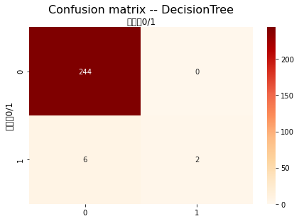
1 2 3 4 'int' ),y_predict_dt)
array([[244, 0],
[ 6, 2]], dtype=int64)
1 2 'Confusion matrix -- DecisionTree' )
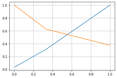
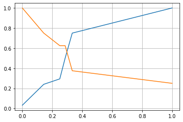
1 2 3 4 5 y_probabilities = dt_clf.predict_proba(X_test)[:,1 ]from sklearn.metrics import precision_recall_curve'int' ),y_probabilities)
1 2 3 4 plt.plot(thresholds,precisions[:-1 ])1 ])
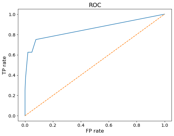
1 2 3 4 5 6 from sklearn.metrics import roc_curve'int' ),y_probabilities)
1 2 3 4 from sklearn.metrics import roc_auc_score 'int' ),y_probabilities)
0.8539959016393442
决策树模型的得分为0.85399 1 2 3 'X0' ,'X1' ,'X2' ,'X3' ,'X7' ,'X8' ,'X9' ,'X10' ,'X13' ],axis=1 )
X4
X5
X6
X11
X12
X14
0
8
0.80
26.16
0
0
0.940725
1
1
0.75
3.94
0
0
0.886500
2
11
0.80
11.41
0
0
0.800570
3
12
0.80
11.41
0
0
0.800570
4
6
0.80
25.90
0
0
0.800382
1 2 3 4 5 6 7 8 9 from sklearn.model_selection import train_test_split'X14' ]for x in data5.columns if x != 'X14' ]]0.2 , random_state = 2020 )
1 2 3 4 5 from xgboost.sklearn import XGBClassifier
1 2 3 4 5 6 7 8 9 10 11 12 13 14 15 16 17 18 19 from sklearn import metricsprint ('The accuracy of the Logistic Regression is:' ,metrics.accuracy_score(y_train,train_predict))print ('The accuracy of the Logistic Regression is:' ,metrics.accuracy_score(y_test,test_predict))print ('The confusion matrix result:\n' ,confusion_matrix_result)8 , 6 ))True , cmap='Blues' )'Predicted labels' )'True labels' )
1 2 3
1 2 3 4 5 6 7 8 9 10 11 12 13 14 15 16 17 18 19 from sklearn.model_selection import GridSearchCV0.1 , 0.3 , 0.6 ]0.8 , 0.9 ]0.6 , 0.8 ]3 ,5 ,8 ]'learning_rate' : learning_rate,'subsample' : subsample,'colsample_bytree' :colsample_bytree,'max_depth' : max_depth}50 )3 , scoring='accuracy' ,verbose=1 ,n_jobs=-1 )
1 2 3 4 5 6 7 8 9 10 11 12 13 14 15 16 17 18 19 20 21 22 23 24 0.6 , learning_rate = 0.3 , max_depth= 8 , subsample = 0.9 )print ('The accuracy of the Logistic Regression is:' ,metrics.accuracy_score(y_train,train_predict))print ('The accuracy of the Logistic Regression is:' ,metrics.accuracy_score(y_test,test_predict))print ('The confusion matrix result:\n' ,confusion_matrix_result)8 , 6 ))True , cmap='Blues' )'Predicted labels' )'True labels' )
大家可以根据以下链接下载信息素养大赛校赛题,每年大同小异,考的基本都是那些,本人在21年参加素养大赛校赛时是刷的20年的题,适用。https://pan.baidu.com/s/1svu1k3AfeZfvsHoTbAs_eg